CCLEX Splat Pipeline

STEP 1

Inspect the capture

Source 2024-ph-cebu-cclexbridge-teleport-knut202609.ply: 638 MB, 2,703,173 Gaussians, full spherical harmonics (3 bands), exported from Varjo Teleport. splat-transform --stats plus a few numpy percentiles showed what we were dealing with:

Finding	Numbers	Consequence
Compact scene	90% of Gaussians within 2.6 km of the centre (units are metres)	crop to a sphere
Sky shell	~3% between 400 and 600 km away	background from the capture app: remove
Near-transparent	683,000 (25%) under 2% opacity	invisible weight: remove
Very large splats	~18,000 over 15 m, most at sea level	keep the sea, drop the ones in the air
Orientation	stored "z-down"	rotate for y-up web viewers

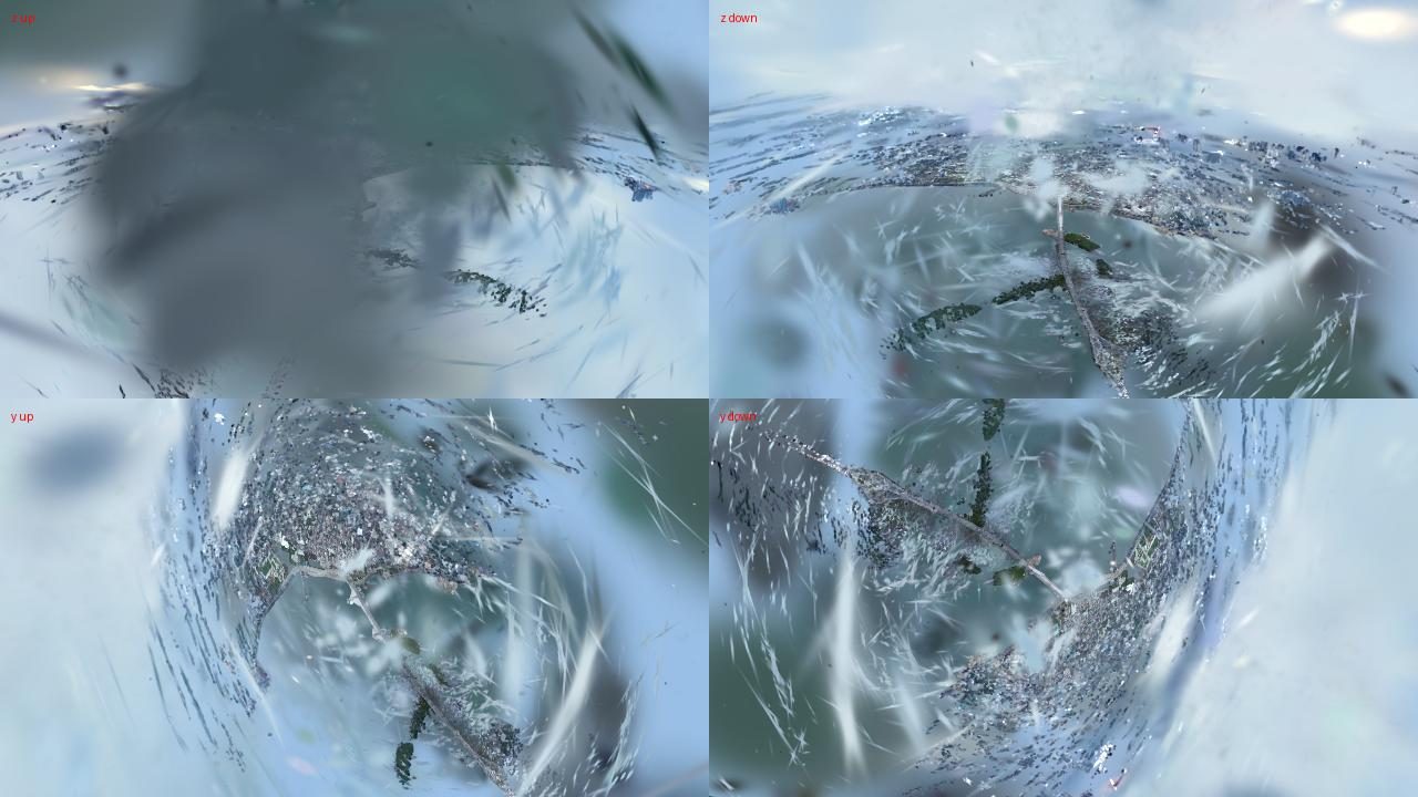
Four test renders of the raw splat from different up-axes — Raw splat rendered with four candidate up-axes. Top right ("z down") is the real aerial view; the streaks in every view are floaters and the far sky shell.

STEP 2

Remove sky shell, haze and floaters

First pass with splat-transform: drop invalid and < 1% opacity Gaussians, crop to a 6 km sphere, drop splats larger than 15 m or 40 m.

splat-transform in.ply -N -V opacity,gt,0.01 -S -63,-62,118,6000 \
  -V scale_0,lt,15 -V scale_1,lt,15 -V scale_2,lt,15 test.sog

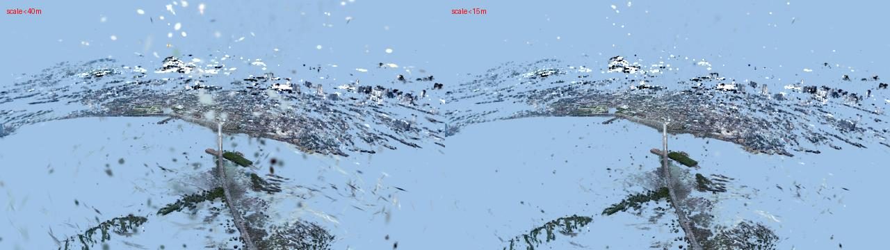
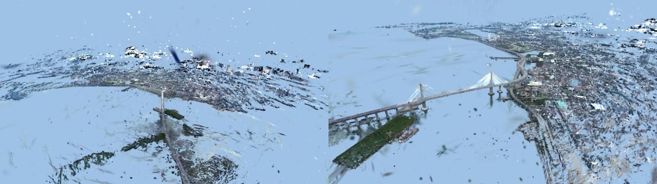
Two renders comparing 40 m and 15 m splat-size limits — Much cleaner, but the sea vanished: the water surface itself is made of big flat splats.

splat-transform's filters can only combine with AND, so the final rule was written in numpy: keep big splats only inside the sea-surface band (z 110–150, found from a histogram of the big splats), drop them everywhere else.

python clean_splat.py in.ply clean.ply --radius 6000 --center -63,-62,118 \
  --max-scale 15 --band-axis z --band 110,150 --band-max-scale 300

Renders with the sea kept and the floaters removed — Sea back, floaters gone: 2,031,179 Gaussians kept (75%). Right: both pylons and the cable fans.

STEP 3

Get the orientation right (and the mistake on the way)

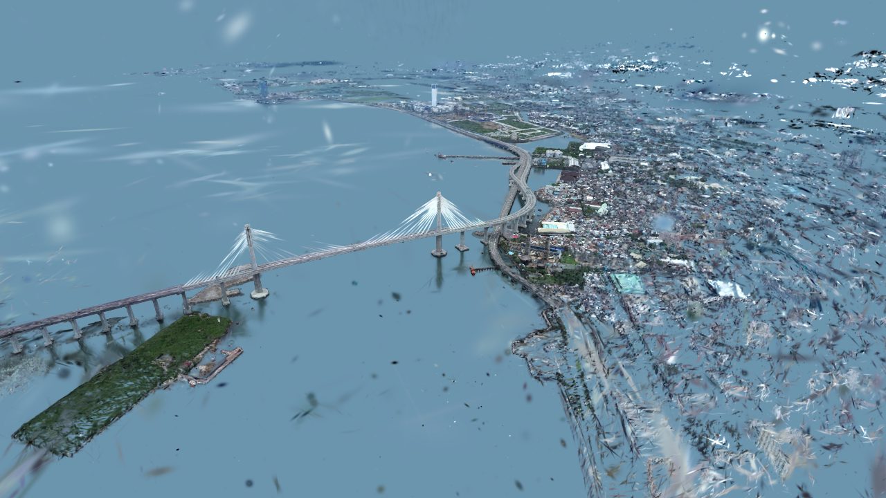
Web viewers expect y-up, so the file was rotated 90° about X. To double-check, I measured heights, and the numbers said the scene was upside down. They were wrong: water reflections are stored as real geometry, a mirror-image bridge below the sea surface, so "most points below the surface" looked like up was down.

Six renders of the mirror-image scene — After the "correction" the cameras were looking at the mirror world: pylons hanging downwards. The first rotation (+90° about X) was right all along.

Lesson. Judge orientation from renders, never from height statistics alone. A camera under the water with a flipped up-vector can also produce a convincing but mirrored aerial view; check left/right against a map.

STEP 4

Compress to SOG

splat-transform clean.ply -r 90,0,0 yup.ply
splat-transform yup.ply -m cclex-bridge-cebu.sog                      # 29 MB, full colour detail
splat-transform yup.ply -H 1 --decimate-adaptive 1000000 m.ply
splat-transform m.ply -m cclex-bridge-cebu-mobile.sog                 # 14 MB for phones

Opening view of the cleaned and compressed CCLEX splat — The 29 MB scene from the viewer's opening camera: Cebu City and the Il Corso tower, the cable-stayed main span, the Mactan shore.

STEP 5

Viewer and portfolio site

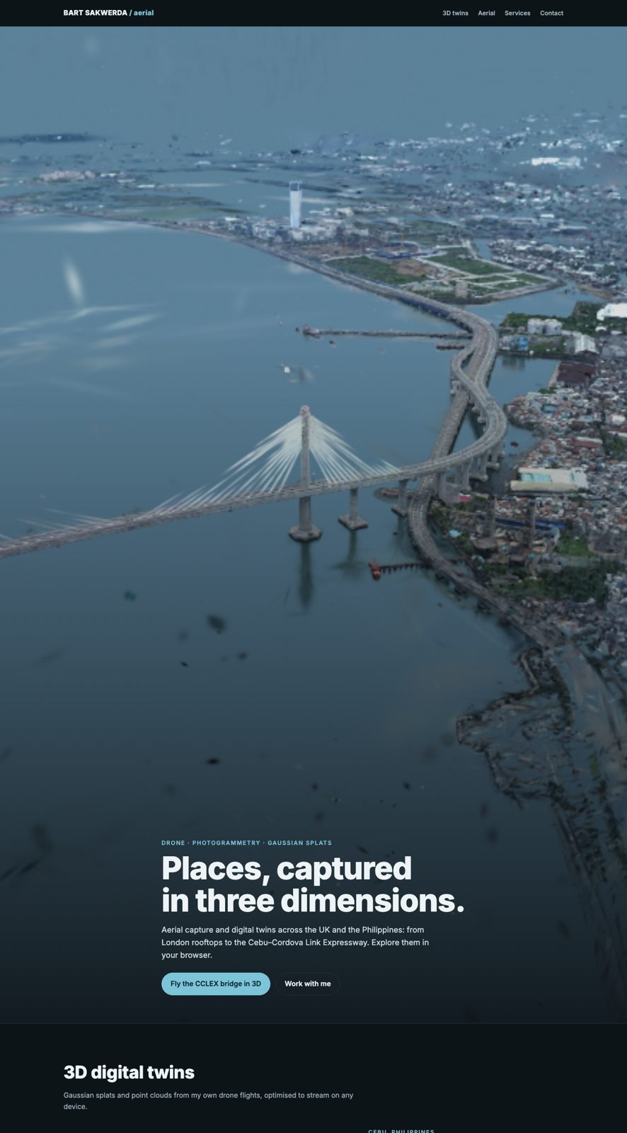
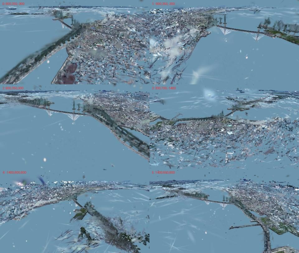
splat-transform cclex-bridge-cebu.sog --unbundled index.html builds a SuperSplat viewer page. Edits: opening camera (renderer coordinates) (-900, 350, 300) → (0, -100, 0), fov 55, background blue-grey so the semi-transparent sea reads as water, and a tiny script that loads the 14 MB file on phones. The portfolio lives on disk7aerials _PORTFOLIO-drones-bartsakwerda/site/ (backup on the Samsung).

Screenshot of the drone portfolio home page — Portfolio home page (desktop, top half). Placeholder boxes show their pixel size until the real images go in.

STEP 6

Segmentation with SAM 3

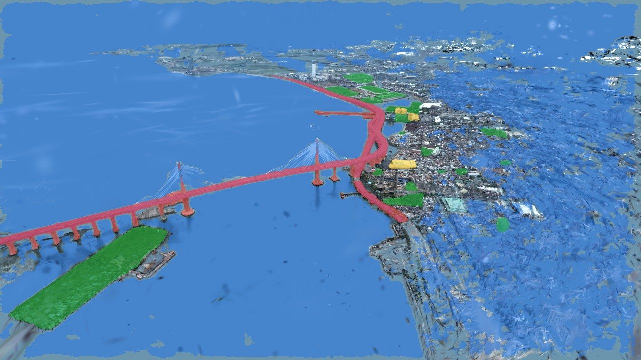
Splat-native segmentation models are trained on indoor scans, so for aerial splats the practical route is: render views, segment them in 2D, vote the labels back onto the Gaussians. SAM 3 runs locally through Apple's MLX (mlx-community/sam3-image): about 10 s for the first image pass, then under 3 s per text prompt.

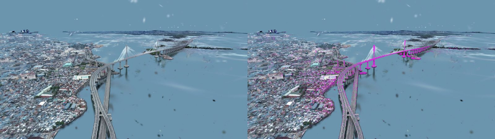
SAM 3 masks on a splat render — Text prompts on one render: red = bridge (deck, pylons, piers, approach in one mask, score 0.79), blue = water, green = vegetation (mangrove island, parks), yellow = houses. Blurry floater areas over the city edge get read as water.

To vote labels onto the Gaussians, their centres are projected into each rendered view with a depth test. The first check failed: the dots did not line up. The cause was that splat-transform's renderer shows the file rotated 180° about Z; with that flip the projection matches (correlation 0.43 against ~0 for every other option).

Projected Gaussian centres over a render — Projection check after the fix: magenta dots (visible Gaussian centres) sit on the deck, pylons, piers and city. The full run labels every Gaussian from 60 views.

STEP 7

Blender digital twin

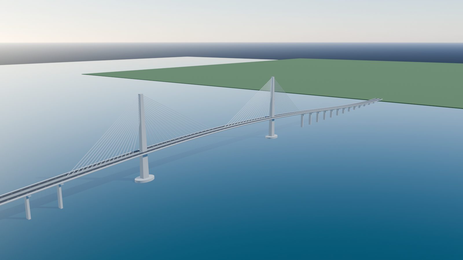
A parametric model built by script in Blender 5.2 from the public dimensions: 390 m cable-stayed main span, two 145 m pylons, 51 m navigation clearance, 27 m four-lane deck (8.9 km total length). Assumed: 150 m back spans, single central pylon column and cable plane (as in the scan), 16 stays per side, piers every 45 m. The scan's centres are included as a hidden reference layer for alignment.

SIDE STEP

Point-cloud pilot (PDAL)

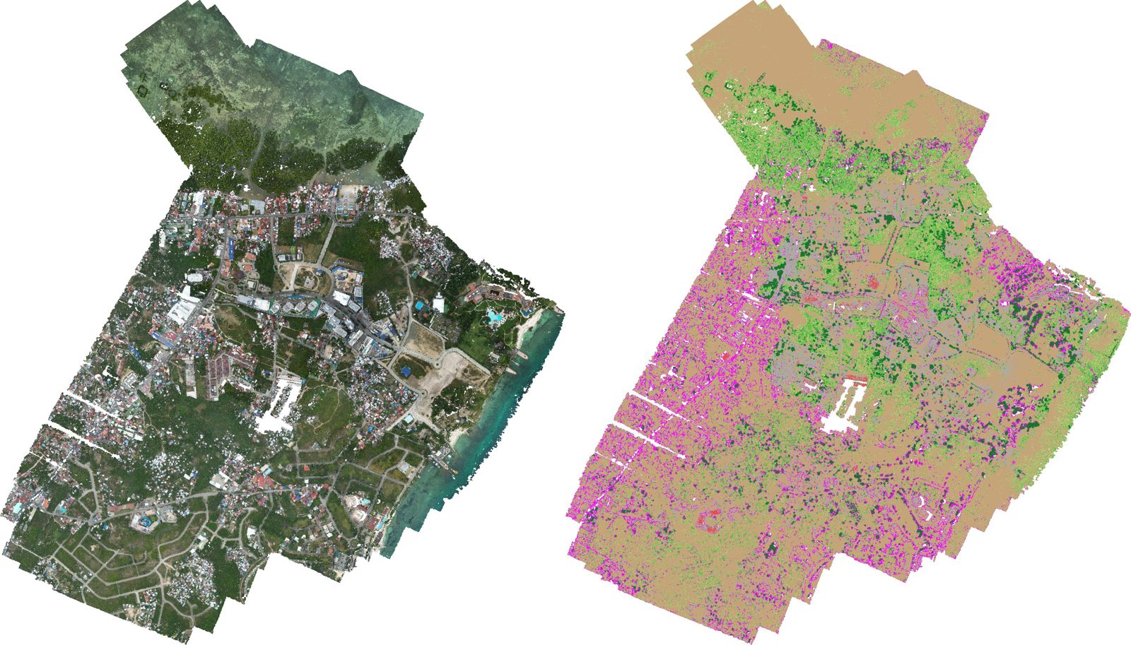
On a Pix4D point cloud of Lapu-Lapu / Mactan (18.8 M points) a rule-based PDAL pipeline (outliers → SMRF ground → height above ground → greenness and coplanarity) ran in under 3 minutes and wrote a classified LAZ 72% smaller than the LAS.

Point cloud photo colours next to automatic classes — Vegetation follows the mangroves and tree lines well; dense low-rise roofs mostly end up as ground or noise, and there is no water class. Buildings need a trained model (Myria3D or SAM lifting).

Lessons and where things are

Lesson	What to do
Capture apps add a far sky shell	crop to a sphere from percentile distances
25% of Gaussians can be invisible	`-V opacity,gt,0.01` (linear scale)
Sea and floaters are both big splats	drop big splats only outside the surface band (numpy OR rule)
Reflections are mirror geometry	judge orientation from renders; check for mirroring
Renderer = file rotated 180° about Z	apply it in any projection; cameras are in renderer coordinates
Capture-app terms and privacy	check Varjo/Luma/Postshot export rights; blur people and number plates

Reusable. The whole workflow is saved as the Claude Code skill gaussian-splat-pipeline (~/.claude/skills/) with clean_splat.py, seg_lift.py and a Blender bridge-twin template.